Note
Click here to download the full example code
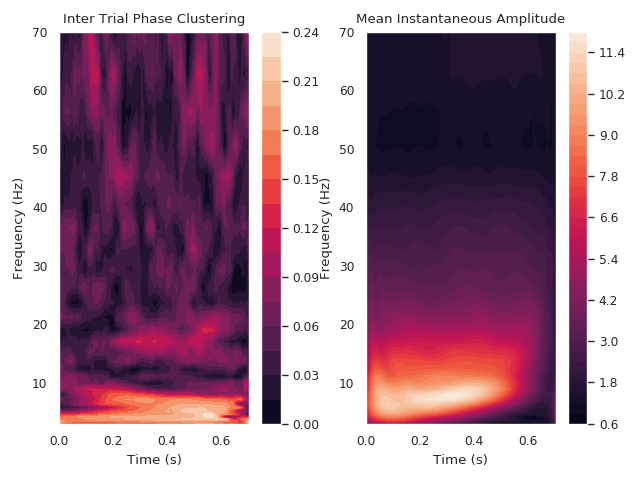
Inter-Trial Phase Clustering
This example shows how to compute and plot the ITPC : Inter-Trial Phase Coherence from a SabDataset instance
# import matplotlib
# matplotlib.use('TkAgg')
import numpy as np
import matplotlib.pyplot as plt
from os.path import isdir, join
plt.rcParams['image.cmap'] = 'viridis'
from sab_dataset import *
import seaborn as sns
sns.set()
sns.set_context('paper')
Load the data : sab dataset
sab_dataset_dirpath = join('pySAB', 'sample_data') if isdir('pySAB') else join('..', '..', 'pySAB', 'sample_data')
sab_dataset_filename = 'sab_dataset_rec_subject_id_040119_1153.p'
rec_dataset = load_sab_dataset(join(sab_dataset_dirpath, sab_dataset_filename))
Print dataset information
print(rec_dataset)
Out:
SAB dataset REC - subject_id
7 channels, 359 points [-0.10, 0.60s], sampling rate 512.0 Hz
356 trials : 183 hits, 173 correct rejects, 0 omissions, 0 false alarms
Channel Info : 7 channels and 1 electrodes
7 EEG channels - 0 non-EEG channels
1 EEG electrodes - 0 non-EEG electrodes
Downsample the dataset
rec_dataset.downsample(2)
Out:
New sampling rate is 256.0
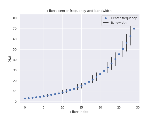
Select filter center frequencies and filter bandwidth
n_filters = 30
filt_cf = np.logspace(np.log10(3), np.log10(70), n_filters)
filt_bw = np.logspace(np.log10(1.5), np.log10(20), n_filters)
f = plt.figure()
ax = f.add_subplot(111)
ax.scatter(np.arange(n_filters), filt_cf, zorder=2)
ax.vlines(np.arange(n_filters), filt_cf-filt_bw/2, filt_cf+filt_bw/2, zorder=1)
ax.set(title='Filters center frequency and bandwidth', xlabel='Filter index', ylabel='(Hz)')
plt.legend(['Center frequency', 'Bandwidth'])
Compute and plot the ITPC of channel 4, for hits trials
rec_dataset.plot_itpc(4, rec_dataset.hits, filt_cf, filt_bw, n_monte_carlo=1, contour_plot=1)
Total running time of the script: ( 0 minutes 34.629 seconds)