Phase basic functions¶

This example shows how to use the Phase functions

# import matplotlib
# matplotlib.use('TkAgg')
import matplotlib.pyplot as plt
from os.path import join, isdir
import seaborn as sns
from phase_utils import *
sns.set()
sns.set_context('paper')

Parameters

fs = 256
tmax = 0.7
data_dirpath = join('pySAB', 'sample_data') if isdir('pySAB') else join('..', '..', 'pySAB', 'sample_data')

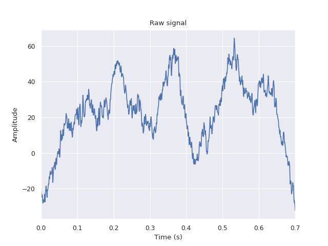
Load the example EEG signal and visualize it

x = np.fromfile(join(data_dirpath, 'rec_042_chan_EEG_Cp1-Cp2_trial_1_2048Hz.dat'))
f = plt.figure()
ax = f.add_subplot(111)
plt.plot(np.linspace(0, tmax, len(x)), x)
plt.autoscale(axis='x', tight=True)
ax.set(title='Raw signal', xlabel='Time (s)', ylabel='Amplitude')

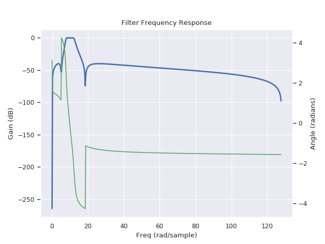
../../_images/sphx_glr_plot_phase_example_1_001.png

Filter the signal in the alpha band bp_filter_1d() allows to visualize the bode diagram of the filter

x_alpha, _ = bp_filter_1d(x, fs, ftype='elliptic', wn=2 / fs * np.array([8, 12]), order=3, do_plot=1)

../../_images/sphx_glr_plot_phase_example_1_002.png

Plot the analytical signal

plot_analytical_signal(x_alpha, fs)

../../_images/sphx_glr_plot_phase_example_1_003.png

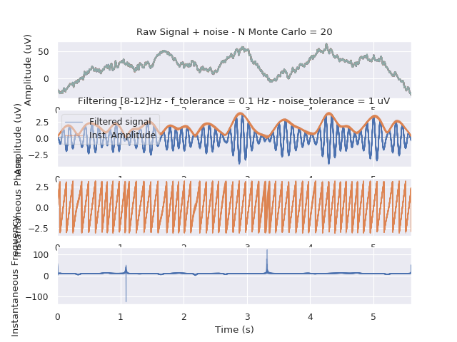
Compute the robust phase estimation

compute_robust_estimation(x, fs, fmin=8, fmax=12, f_tolerance=0.1, noise_tolerance=1, n_monte_carlo=20, do_fplot=0,
                          do_plot=1)

../../_images/sphx_glr_plot_phase_example_1_004.png

Total running time of the script: ( 0 minutes 0.428 seconds)

Gallery generated by Sphinx-Gallery