Note
Click here to download the full example code
Feature Evolution and Distribution
This example shows how to plot feature evolution, or the distribution of a feature over trials at a certain time point.
# import matplotlib
# matplotlib.use('TkAgg')
from os.path import isdir, join
import sab_dataset
import seaborn as sns
sns.set()
sns.set_context('paper')
Load the data : sab dataset
sab_dataset_dirpath = join('pySAB', 'sample_data') if isdir('pySAB') else join('..', '..', 'pySAB', 'sample_data')
sab_dataset_filename = 'sab_dataset_rec_subject_id_040119_1153.p'
rec_dataset = sab_dataset.load_sab_dataset(join(sab_dataset_dirpath, sab_dataset_filename))
Downsample the data
rec_dataset.downsample(2)
Out:
New sampling rate is 256.0
Construct the features from the SabDataset object - Select only ‘hits’ and ‘correct rejects’ trials and keep only 2 electrodes of interest :
time_features = rec_dataset.create_features(trial_sel=(rec_dataset.hits | rec_dataset.correct_rejects))
print(time_features)
Out:
Time Features subject_id_rec - 7 features, 180 time points, 356 trials
2 labels : {1: 'Hits', 2: 'Correct rejects'}
Feature types : Amp
Extract features, if called without any parameter, the function return the possible feature to extract
time_features.extract_feature()
Out:
Possible features to compute : ['filt_bandpower', 'dwt', 'stft_bandpower', 'stft_phase', 'cwt_bandpower', 'cwt_phase', 'phase_hilbert']
Extract the discrete wavelet transform coefficients, The new features are automatically added
time_features.extract_feature('dwt')
print(time_features)
Out:
Time Features subject_id_rec - 42 features, 180 time points, 356 trials
2 labels : {1: 'Hits', 2: 'Correct rejects'}
Feature types : Amp, DWT 4-8 Hz, DWT 8-16 Hz, DWT 16-32 Hz, DWT 32-64 Hz, DWT 64-128 Hz
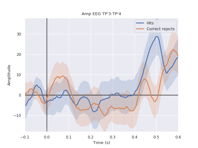
Plot the evolution of feature 19 :
time_features.plot_feature_erp(feature_pos=2)
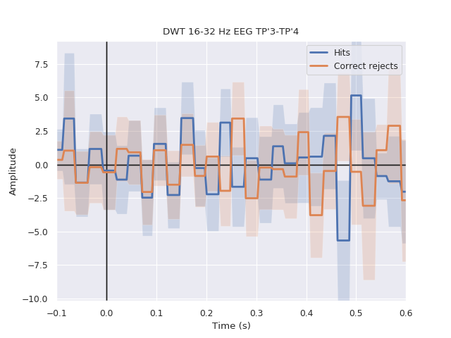
Plot the evolution of feature DWT 16-32 Hz for channel TB‘10-TB‘11 :
time_features.plot_feature_erp(feature_type='DWT 16-32', feature_channame='EEG TP\'3-TP\'4')
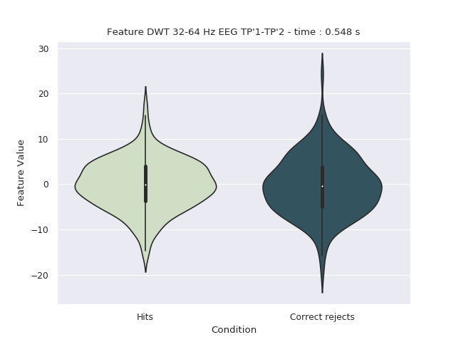
Plot the distribution of a feature at a certain time point. The ‘time_points’ parameter must be passed and contain only 1 time point
time_point_sel = time_features.time2sample(0.55)
time_features.plot_feature_distribution(time_points=time_point_sel, feature_pos=10)
Total running time of the script: ( 0 minutes 0.736 seconds)