Note
Click here to download the full example code
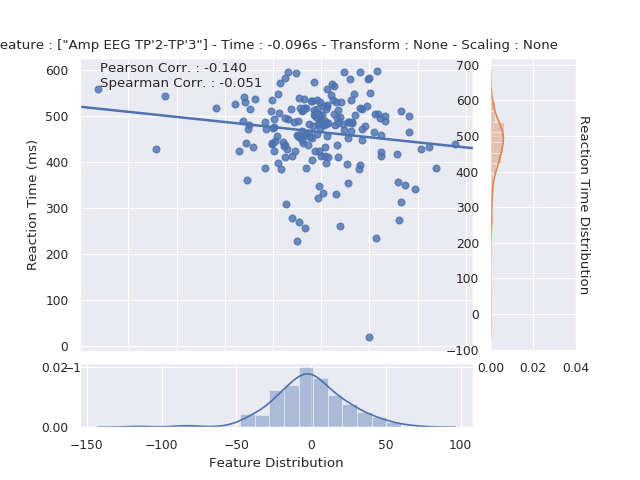
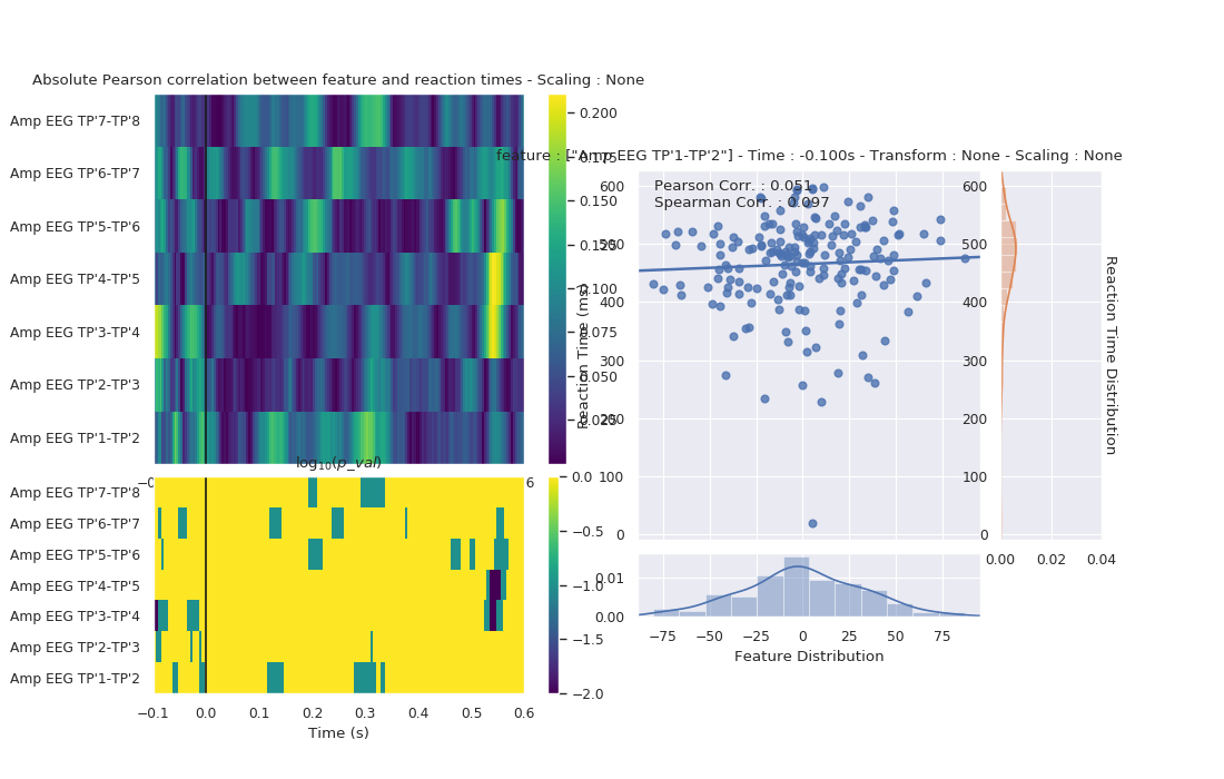
Hits / Reaction times correlation
This example study the correlation between the Hits features and the reaction times.
# import matplotlib
# matplotlib.use('TkAgg')
from os.path import isdir, join
import matplotlib.pyplot as plt
import sab_dataset
import seaborn as sns
sns.set()
sns.set_context('paper')
Load the data : sab dataset
sab_dataset_dirpath = join('pySAB', 'sample_data') if isdir('pySAB') else join('..', '..', 'pySAB', 'sample_data')
sab_dataset_filename = 'sab_dataset_rec_subject_id_040119_1153.p'
rec_dataset = sab_dataset.load_sab_dataset(join(sab_dataset_dirpath, sab_dataset_filename))
Downsample the data
rec_dataset.downsample(2)
Out:
New sampling rate is 256.0
Construct the features from the SabDataset object - Select only ‘hits’ and ‘correct rejects’ trials and keep only 2 electrodes of interest :
time_features = rec_dataset.create_features(trial_sel=(rec_dataset.hits | rec_dataset.correct_rejects))
print(time_features)
Out:
Time Features subject_id_rec - 7 features, 180 time points, 356 trials
2 labels : {1: 'Hits', 2: 'Correct rejects'}
Feature types : Amp
Extract features, if called without any parameter, the function return the possible feature to extract
time_features.extract_feature()
Out:
Possible features to compute : ['filt_bandpower', 'dwt', 'stft_bandpower', 'stft_phase', 'cwt_bandpower', 'cwt_phase', 'phase_hilbert']
time_features.plot_feature_hits_reaction_time(time_points=1, feature_pos=1)
time_features.interactive_feature_rt_correlation(feature_channame='TP\'')
plt.gcf().set_size_inches(11, 7)
Total running time of the script: ( 0 minutes 0.580 seconds)